Okay 1am here bed now but all yesterday I spent investigating materialization, where what I’m learning about that has led me into a quick check/investigation into what happens when a merge join is running on a table which is less than 100% sorted.
My particular test scenario right now is three nodes of dc2.large, so six slices. I give each slice an equal number of rows and then fully unsort one slice with an update.
This gives me about 15% unsorted rows - so I still get a marge join, according to explain plan.
So, wanna know the kicker?
With a 100% sorted table, I get a merge join - simple. That’s it.
With my test table, I GET A SORT STEP BEFORE THE MERGE JOIN.
Holy cow on a stick.
The query plan is completely unchanged - identical in both cases.
I need tomorrow to check what happens when I have, say, six slightly
unsorted slices (rather than a single fully unsorted slice), but my
guess right now - if you’re less than 20% unsorted (according to
SVV_TABLE_INFO, which to my eye has a crazy way of computing how sorted
tables are), then you get a sort step. If you’re more than
20% unsorted, you get a hash join.
So, folks, being a “bit unsorted” in fact really matters. You need to be 100% sorted to get a pure, maximum efficiency merge join, especially since that sort stage with any reasonable data or with a slot which has almost no memory (because 100% merge joins simply do not use memory and the slots may be set up for that) is going to sort on disk.
I think I’ve finished investigating - there was actually only one more test that had to be performed to answer all the questions I currently have.
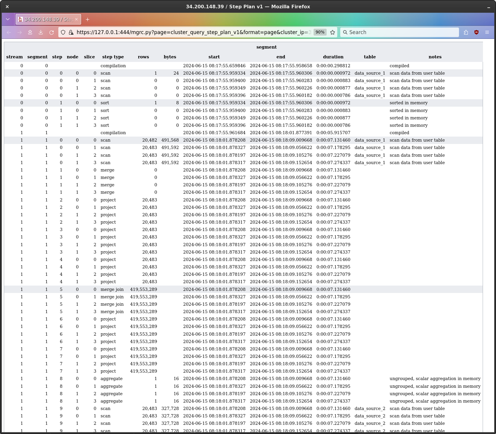
So I made two tables, identical, and then unsorted one row in one of the tables.
Bingo - sort step turns up.
But! get this - the sort step sorts ONLY THE UNSORTED ROWS.
(I’ve highlighted the steps where the single unsorted row is being handled.)
Yes! so in fact what’s happening is this : scan the sorted region from both tables, scan the unsorted region, sort the unsorted region, and then - mmm - and then what?
Looking at the step plan we see a merge step - but it has 0 rows on all slices, which makes it look like a no-op. If it was actually merging the sorted region and the now-sorted unsorted region, I’d expect to see a row count.
So, I think one of two things is happening.
In any event, the biggie is this : if you’re not 100% sorted, you get a sort step before your merge join.
I’ve long wondered how the merge join handled the up-to-20% unsorted
region. As an aside, if SVV_TABLE_INFO says 20% unsorted,
you get a hash join. You need to be less than, not less than or
equal to, 80% sorted. I tried to find the official docs page on merge
join, but failed (it did exist once - I’ve read it in the past), so I
can’t post a URL or quote.
Well, folks, this is an important blog post.
I’ve spent three full days investigating materialization, which is to say, Redshift is a column-store relational database, but of course it emits rows, and so at some point those columns have to be joined back into rows, where this process of rejoining columns to form rows is called materialization, and I finally now fully understand (or at least, everything makes sense, is internally consistent, and I make correct predictions) what’s going on.
The work will end up being a PDF, but no time for that ATM, so blog post for now.
So, where to begin.
In a conventional relational database, we can say that each table is stored in one file, but that in a column-store database, each column is stored in one file.
When rows are provided to the database to be added to a table, they are normally provided as contiguous rows, and these rows necessarily then are broken up into columns so each column can be appended to the file for that column. That’s fine, straightforward.
What’s much more interesting, and trickier, and very important to understand with regard to performance, is what happens when a query comes along and wants to read a table, because if that query is going to use more than a single column, we need to join columns back together, so we can emit rows.
Let’s say we have a single table, ten columns, and a query comes along and wants to use say five of those columns - let’s say two columns are in the where clause and so then are deciding which rows are read, and the other three columns are in the select clause, and so actually form the rows which are produced.
Now, there’s a couple of ways you could immediately think about how to approach this problem.
What immediately comes to my mind is that you start reading the two columns which decide which rows to select, and only read the other three columns when you have a row you’re going to keep - so you’d be scanning down the first two columns, you’re find a row you want to keep, and of course you inherently know the row number you’re on, so you compute the offset of the value you want in the files for the three columns in the select, and so get the values for the row, and voila! there’s the row.
There’s a couple of problems with this approach.
First, you’re going to do a lot of disk seeks. That’s a complete massive no-no for performance. Death on a stick. Completely off the menu. (Also, Redshift just doesn’t work this way - all disk I/O is in one megabyte blocks - but that’s by-the-by for now; I’m currently discussing broad principles, not RS).
Second, this approach only works if the length in bytes of each value
in the three select columns is always the same. If the length
is always the same, then we can directly compute the offset of
the value we want (row number times value length), but if the value
length varies by value (a varchar or varbyte),
or maybe we have data compression in play, then we can’t. No
bueno. Can’t work.
However, regardless of the issues with this approach, what I can say to you is that this is an example of what is known as late materialization, which is to say, you defer joining up rows until you know you actually need a row.
There is an alternative approach, which is known as early materialization.
What we could do - and we’d need some extra information available to us to do so, but we’ll come to that - is first materialize every single row which the query could possibly read, and then having done so actually now go and look at the actual values in those rows and figure out which rows we’ll actually keep.
So late materialization we can consider minimalist, and early maximalist.
Now you might think, well why on earth would anyone take this approach when it’s obviously so much less efficient? and the answer is : it can be the right choice in the situation the developers are in at the time they come to decide which approach to use.
What I mean by this is that Redshift (superb name, highly successful product) came from ParAccel (terrible name, totally failed product, just sayin’ :-), which in turn came from Postgres 8 - and Postgres is a conventional, row-store database.
I don’t know this for a fact, I’ve not spoken to any of the devs involved, but given that the Postgres database engine is row-store, I think when the devs came to decide to add column-store to Postgres, it was going to be much, much, much easier to bolt column-store “on the side”, by making it present fully formed rows to the row-store database engine, than it would be to modify that database engine to be genuinely implement column store and so have to know all about columns.
In any event, Redshift does use early materialization, and I will now describe the implementation.
Now, when Redshift comes to read a table, there is a
scan step (queries are broken down by Redshift into
streams, segments, and steps - go read say the Serverless PDF to get an
explanation of all that).
It turns out the scan step in fact has two stages; where
the first stage turns out to be using and only using the information
available in STV_BLOCKLIST, which is to say, information
about and only about blocks (minimum and maximum value per block, and
number of rows in a block), and that first stage materializes all the
rows which the query could possibly read, and then having done so the
second stage then occurs, and now Redshift goes and look at the actual
values in the materialized rows and figures out which rows we’ll keep,
and it is those rows, from the second stage, which are emitted
by the scan step.
So stage one is block information only - absolutely no looking at the values in the columns - and then stage two takes the rows materialized by stage one and actually looks at the values in the columns.
Now, remember here that all disk I/O in Redshift is in one megabyte blocks. No exceptions. This is a Big Data database. We are not at home for Mr. Single Row Please.
Also, particular point to remember here - I am here talking about and only about reading a single table. I am not talking about joins. I’ll get to them once I’m done talking about a single table, and explain how they fit in and what’s happening with them. So, right now - single table only. Remember that, and put joins to one side for now.
So, when a query is issued which reads a table, for every column in the where clause which has a value actually specified (e.g. colour = ‘blue’, age = 10, latency > 150, etc, etc), Redshift can directly see which blocks in that column could contain that value (because the value falls between the minimum and maximum value for a block in that column).
Now, remember, in the first stage, Redshift is not looking at the values in rows. It is and is only using block information.
At this point, Redshift now knows for every column which has a value specified in the where clause which blocks could contain the values specified in the where clause, which gives us what we need next - which is what is known as the row range for each contiguous set of blocks (and that might be a single block only, which is fine), which is to say the start and end row number of each block, which Redshift knows because it knows how many rows are in each block (and so it can directly compute the start and end row number for any block).
So now with the row ranges for each where column in hand, Redshift performs what is known as inference, to reduce if possible the number of rows which have to be materialized.
What Redshift does now is examine the logic of the where clause.
Imagine we have a where clause which states colour = ‘blue’ and age = 10.
Note the and. Both conditions must be true.
Redshift currently has row ranges for the first column, for all rows
which could be blue. Redshift similarly has the row ranges
for the second column, for every row which could be 10.
The logic in the where clause says and. Rows must be both blue and 10.
So if we have a range of rows in the first column which has no matching range of rows in the second column, we can know it cannot be used by the query. Bingo - we can cull such ranges of rows.
This is done, far as I can tell, for all row ranges in all columns, no matter how many separate row ranges there are, but I’ve not particularly tried to test this to see how far it goes. I imagine internally there won’t be a limit, it’s not hard to imagine ways to do this which work for any number of row ranges.
Finally now we have the list of row ranges to be materialized.
Now, at this point, there is something which isn’t clear to me.
Right now, we’ve reached the very end of the first stage - we know, from block information only, which rows we need to materialize.
Question is, do we materialize - actually produce on disk - all these rows, and then look at their values to see which rows we’re really going to keep (i.e. if the query says it wants all rows which are age = 10, but we read a block which has a bunch of rows where age = 9 or age = 11, we need to keep only the rows where age = 10, and that now means we actually finally look at the values in the rows, which we were not doing before; before it was block information only), or, when we come to materialize on disk, do we examine the values in the rows and actually produce (emit to our output) rows which the query needs?
I don’t know.
But I do strongly suspect, but again do not know, that the rows we do
emit are in fact materialized into row-store tables - on worker
nodes! - which are then used by Redshift for further query work. So I
think after scan, we’re no longer working with blocks.
We’re back to actual rows.
So, so far, so good. Now we have a picture of what’s going on under the hood.
Now for the stuff you have to worry about - and by that, I mean data compression.
So, I’ll start with a simple example to illustrate the problem that can occur with data compression.
Imagine you have a query which specifies a single value in a single column, and in fact there happens to be in that table just the one row with that value (that it’s a single row is not necessary for the problem I’m describing - it just particularly highlights the problem).
So in the query we specify in the where clause that the column needs to equal, say, 100, and there is only one row with that value.
Now, that column turns out to be very highly compressed - let’s say
zstd with lots of repeating values.
As such, the single block which contains the single row with that
value in fact contains millions of other rows - with
zstd and say int8, you can get eight million
rows in a block, no problem.
Redshift now knows the one block which contains that value, and the number of rows in that block is huge - millions - and every single damn one has to be materialized.
Bugger.
Having then materialized those rows, the values in them are now
actually read, and we finally find the one row with value 100, and that
single row is now returned by the scan step.
Regardless of whether or not Redshift is actually materializing all those rows, or only the single row which is emitted, having to iterate over eight million rows is far from ideal.
To provide contrast, imagine we’d had raw compression
and int8. This would give us 130,944 rows in that block,
and we’d materialize only those 130,994 rows. Sure beats eight million -
but of course it’s not really like that. To do this, you’ve given up
compression, and as we will see, in fact, most of the time this problem
simply isn’t happening and you can - and most definitely should,
compression is great for performance, because it reduces disk I/O so
much - keep compression.
Now we actually understand what’s going on, we can safely read the advice AWS give in this matter - or we could, if I could find it. I can almost never re-find material I’ve in the past read in the docs.
In any events, what was written was something like;
Always use raw encoding for the first compound sortkey column.
What’s actually going on here are a couple of assumptions and then playing safe always, no matter what, but at very considerable cost.
The first assumption is that you will be specifying values for the
first compound sortkey column in the where clause (on the basis that it
is the first sortkey column), then, secondly, that because the
column is the first sortkey column, it will compress highly, and so then
with both these assumptions true it would be possible for the
problem described above to occur - and so the advice is let’s
always avoid it by using raw encoding, despite its
huge cost when this problem is not occurring, which is in fact the
normal case.
(And in fact, the auto encodings select raw for
all sortkey columns, not just the first. Go to town, why
not.)
The problem with all this is that it’s often not a problem, and playing safe can be expensive.
Imagine I’m querying a not one row of data, but a month of data - something much more normal on Redshift, which is for Big Data and analytics. The sortkey for this imaginary table is the date of the row, and I’m issuing a query where in the select clause I’m selecting one other column (not the sortkey).
So one column in the where clause (and it’s the single sortkey), and one column in the select clause (not the sortkey).
So let’s say we have the sortkey uncompressed. I could well need to
read now a hundred plus blocks of sortkey, where if I’d used
zstd I’d be reading single digits of blocks. Where I’m
reading a month of rows, the select column I’m reading is going to be
compressed, and so it will be a few blocks. I’ve only lost out here by
going for raw on the sortkey - instead of reading single
digit blocks from both columns, I’m now reading hundreds of blocks from
the sortkey. The problem AWS advise against was not present because
there is no significant disparity in the number of blocks and rows used
in these two columns.
That situation is in fact the situation I had with my test data in
this investigation. Rows here means rows evaluated for materialization,
with the actual number of rows returned by the scan step
was 65,497.
So here in this table you can see the problem. There’s a big difference between the AWS recommended encodings (147 blocks) and the correct encodings (29 blocks).
| column_0 | column_1 | rows | blocks |
|---|---|---|---|
| raw | raw | 16,767,232 | 313 |
| raw | zstd | 16,767,232 | 147 |
| zstd | raw | 24,301,557 | 188 |
| zstd | zstd | 24,301,557 | 29 |
Indeed, the problem scenario AWS are looking to avoid, which gives 188 blocks, is improved by the AWS solution by only 41 blocks (down to 147) - but both the problem situation and the AWS solution are over 100 blocks worse than the correct solution. Of course, your mileage will vary depending on your data (although my data was not particularly strange in any way), but it makes a point - what AWS have done is ultra-cautious and costly. This is not good.
However, there is a caveat here. My test code is using at most 313 blocks, on a completely idle two node dc2.large. When I benchmark these queries, they all take about 120ms. Most of that is going to be irreducible overhead - I don’t have a test set up now which works with large enough numbers of rows to be able to tell the performance difference between these four choices.
This is an important open question - everything written so far makes perfect sense, but I need to actually see that the cost of having an extra 8m rows to materialize (24,301,557 vs 16,767,232) is in fact massively outweighed by the benefit of not reading an extra 100+ blocks.
I’m extremely confident this is so, but it needs to be proved. I won’t have time to do so for a little while - days, week - so I’m going with it for now. Just be aware of it and keep an open mind on this one until I have some benchmark numbers.
Also, in particular, that the AWS advice writes about the sortkey, as if it were special, is a red herring. The fact the column is a sortkey is in and of itself meaningless; it’s simply a placeholder for “a column which is highly compressed and used in the where clause”. There are a lot of columns which are like that, not just sortkey columns, and of course then even when such columns are used in the where clause, we must then examine the select columns to see if we actually have a problem at all anyway.
The simplest worst case scenario for this is when you have a single
actual row being matched, and that row in the where clause is in a
massively compressed column (think az64 in one of its no
less than three different, all mind-bending, run-length
compression modes and you’ve ended up with say more than two billion
(yes, billion, yes I’ve actually done so myself - seen with my own eyes)
values in single block), and then the select column has very few values
per block (varchar(max)) and just for fun is not compressed
either. Now you need to read two billion 65k strings to find one
row.
Moral of this story : understand az64 before you use it
(note that it is the default encoding used by Redshift for everything
except strings and sortkey columns), and don’t use long bloody strings
in Redshift. This is not a use case. All you people importing
SAP data into RS as varchar(max)? find a different
database.
The thought now crosses my mind that SUPER with 16mb
blocks, is going to make this eeeeeeeeeeeven worse. I’ve not
investigated SUPER, so I don’t know how it behaves, but on
the face of it, well, you can see the problem.
We still see some of this problem, but reduced in extent, when both the where and select columns have much the same number of rows per block, but when the row count is high and we’re looking for a single row; the row may well now match only one block in both where and select, but that block may have a lot of values in. That’s still not great.
Basically, the more you compress, the better for disk I/O, which is really, really important - central to everything - but the more you compress, the more single/few row reads become expensive, because you have a lot of rows to process to find the one row you want in the block you’ve read.
This is actually coming back to the fact that Redshift is an analytics database, which is by design intended to be good at handling queries which process large numbers of rows, and by being good at that, inherently becomes poor at handling small numbers of rows.
If you use Redshift for a use case it is not designed for, do not expect it to end well.
This is the second most common thing you’ll hear from me about databases.
The first is : the data in the database will be as wrong as the data types allow it to be.
Coming back to Redshift and its use cases, when you come to design a database and you take the design decisions necessary for the database to be effective at analytics, you necessarily end up being awful when it comes to working with small data (such as single rows).
People assume - and AWS does nothing to correct them - that a database can do anything. I’ve used Postgres, Redshift MUST be able to do all these things! I can issue SQL on Redshift - so it MUST work! the idea that the underlying database engine is profoundly different is not on the menu. Redshift is seen as being Postgres, but bigger, faster, and able to handle Big Data. No one is explaining to them that Redshift is utterly unlike Postgres, and does not overlap, and there’s a whole bunch of stuff they do on Postgres they cannot do on Redshift, even though they could actually issue the queries.
So what Redshift (well, ParAccel, this predates AWS) has done here in its implementation is absolutely right for working with Big Data, and is also inherently and unavoidably wrong when it comes to working with small data. The correct answer here is do not use Redshift for small data. Use a more suitable database technology, such as Postgres.
So, in summary, the problem really is not so much compression, but data - you have data in where columns which is particularly compact, and in select columns which is particularly voluminous. Compression can cause this situation, and certainly can greatly exacerbate this situation, but it’s really in the end about the data in the columns.
So that’s everything for reading a single table.
I said I’d come back to joins.
In Redshift, each table is read (scan step) individually
and independently of all other tables; materialization occurs, and then
the materialized rows are actually examined, and the matching rows from
that table are returned from the scan step (which can of course be all
the rows in that table).
Joins happen after all this, later on in the query, in their
own separate steps, and they work with and only with the rows actually
returned by the scan step (in the what I think are
row-store tables on the worker-nodes, keeping in mind these tables
retain the sorting order of the original table, and so for example merge
joins are no problem, assuming all the usual conditions are met).
Joins are never involved in the work of deciding which rows to materialize. With late materialization, they could be and would be, and you’d get efficiency gains from it. But not in early materialization.
So I want to write a bit about concrete examples for the previous post, about materialization.
Imagine we have a query, one column in the where clause, one column in the select. The where clause is raw encoding, the select column is massively compressed - let’s say zstd with lots of entropy.
By using raw for the select column, we make the row range for the select column as accurate as possible. That’s good. On the downside, and it’s a heavy downside, we now are reading lots of blocks. That’s baaaaaaaaaaad.
The select columns is massively compressed, so we can imagine here that our entire row range from the where column fits into one block, and that block has a bazillion rows.
Now, we in fact have pretty much the minimum possible row range, from the where column, but in most blocks you have to decode the entire block to get to get given row (certainly true for zstd, lzo, runlength, etc) and I suspect RS just does that always.
So we’re going to process, for whatever that means - it’s one of the two open questions - all the rows in that block but only up to the final row in row range. After all, there are no rows we need after the final row in the row range, so we bail out at that point.
I suspect what process means is the block is loaded into memory, is decoded in memory, and here now we’re looking at actual values in the rows, we emit only the rows we care about to our output table. So we process all the rows prior to the start of the row range, then emit all the rows in the row range, and then we’re done.
Processing in memory is pretty darn cheap, but if take something which is pretty darn cheap and multiply by a bazillion, it can become pretty darn expensive.
Now let’s imagine we have one column in the where clause, and two select columns. The where clause is raw still, one of the select columns is super compressed (as before), but the new select column we have now is fairly well compressed. What happens?
So, the row range that we care about always come from and only from the where columns. Select columns play no part in this.
The where column then gives us the row ranges we care about.
Next, we look at the select columns, and we need to get hold the blocks which cover the row ranges.
For the super compressed column, this is one block. For the new second column, where it’s fairly well compressed, let’s say this is five blocks.
We now need to materialize the row range in hand from the single block of the second column, and the five blocks of the third column.
RS reads the blocks, skips the leading rows in the first block from each column when they are not part of the row range, and then once it hits the first row in the row range, gets to work materializing rows,
Next example, what happens when there is no where clause. In this case, there are no where columns, and so the row range is that of the entire table; there’s nothing to make it less.
Then we have a situation with a single where clause which is like this; column_1 = column_2. In this case we do not have literal values available, so we cannot produce row ranges when we materialize, so we materialize every row, and then we keep only the rows where column_1 = column_2. How much work this is, is going to depend very much on whether or not RS actually materializes all rows before looking at values, or if it inspects value while materializing (and I suspect the latter).
One final point which I became more aware of today is that the rows in the where and select blocks could be very highly disordered. IIRC, in the previous post, I wrote something like : we examine the where column(s), produce our row ranges, and then we materialize rows, and in the situation where we have a select block with a bazillion values, and the row range fits entirely inside, and where we know the select column must say equal 10, then once we get to the value 11 we can stop processing (even though we’re still inside the row range).
This is basically wrong. What happened is that the test data I created was ordered in all its columns - I controlled the values in each column, and so even though only the first column was sorted, all the other columns were in fact sorted as well. If we consider a typical table, there are one or two columns in the sortkey, and the other columns are not in the sortkey - and the columns not in the sortkey typically are highly disordered, because the table has been sorted, so all the rows have been moved around, which is usually going to make a mess of columns which are not in the sortkey.
So when we have a row range, and we have a select column with one block with a bazillion rows, we are first of course interested only in the rows which are in the row range, but of those rows, any of them could be the value we’re looking for, because in fact that block is randomly ordered. As such processing always has to cover the entire row range; it can’t finish early.
Jesus. Wow. I have finally found the first actual example of a
profound improvement in query behaviour due to running
ANALYZE. I had a query which was running a distribute step
- an expensive distribute, we’re talking 3.5 billion bytes over
the network - go away after analyze.
Prior to the analyze, the table was missing stats completely.
Just a heads up - the docs describing deep copy, which is the use of
INSERT to a new table, instead of VACUUM - are
flatly wrong.
(I had been wondering why I kept thinking that INSERT to
a new table produces sorted blocks, when it does not.)
https://docs.aws.amazon.com/redshift/latest/dg/performing-a-deep-copy.html
A deep copy recreates and repopulates a table by using a bulk insert, which automatically sorts the table. If a table has a large unsorted Region, a deep copy is much faster than a vacuum. We recommend that you only make concurrent updates during a deep copy operation if you can track them. After the process has completed, move the delta updates into the new table. A VACUUM operation supports concurrent updates automatically.
Deep copy is being presented as a replacement for
VACUUM.
So, here’s how it works.
When you add rows to a table, by whatever means, the incoming rows are sorted with respect to themselves (to help with min-max culling) and then appended to the table as unsorted blocks. They’re unsorted, because they are not sorted with respect to the table as whole.
Now, with COPY, if you add rows to a new or truncated
table, those blocks are added as sorted blocks. If you
COPY into a table with one or more rows already present,
they’re appended as unsorted blocks.
However, with INSERT, the new rows are always
appended as unsorted blocks.
The docs say
A deep copy recreates and repopulates a table by using a bulk insert, which automatically sorts the table.
This is flatly wrong. The table is not sorted. The incoming rows have been sorted with respect to themselves, but even though the table is new, they are still added as unsorted blocks.
Everyone reading the docs is thinking insert to empty table is the
same as vacuum. It is not. To make those blocks sorted, you
need to run VACUUM FULL [table] TO 100 PERCENT; after the
INSERT. BTW, always use 100 PERCENT. The way
Redshift thinks about that percentage is conceptually wrong, and it can
lead to you having a completely unsorted table which VACUUM
tells you is highly sorted.
Now, I would hope that in this situation where the rows are all
sorted and there are no previously existing rows, VACUUM is
smart enough to make this almost a no-op; just mark the blocks as
sorted. Alas, experimentation shows this is not the case; it’s certainly
doing some real work - but it might well still be pretty quick, like
minutes rather than days!)
So, could be, if you’re going to deep copy, you have to do it by
UNLOAD to S3 and using COPY for the load.
(And don’t forget to ANALYZE. New tables have no table
stats. ALWAYS keep table stats up to date, I very strongly expect - but
have not investigated so do not yet know as a fact - they are how hash
joins decide which table is small, and is hashed, and which table is
large, and is iterated over. You do not want that decision
going wrong, because the query may well then overflow memory in its
slot, which means it begins to hammer disk, and then everyone
suffers.)
Home 3D Друк Blog Bring-Up Times Cross-Region Benchmarks Email Forums Mailing Lists Redshift Price Tracker Redshift Version Tracker Replacement System Tables Reserved Instances Marketplace Slack System Table Tracker The Known Universe White Papers